Introduction

Automated System for MPM

AutoMPM is a tool developed for automatic machine learning in Mineral Prospective Mapping (MPM). It provides user-friendly python-based interface for MPM.

AutoMPM stands as an innovative solution, purposefully crafted to revolutionize the landscape of MPM through automated machine learning. In the realm of mineral resource exploration, MPM serves as a cornerstone, pinpointing locales with elevated potential for distinct mineral deposits. Previously, these endeavors demanded laborious, hands-on techniques, characterized by protracted timelines and susceptibility to inherent human inclinations. AutoMPM ushers in a paradigm shift, offering an advanced toolset that streamlines and refines this process with cutting-edge automation.

AutoMPM User Guide

Welcome to the AutoMPM user guide, where we delve into the efficient and automated world of Mineral Prospectivity Mapping. AutoMPM is designed to streamline the MPM process, leveraging advanced machine learning techniques to uncover high-potential mineral deposits. Say goodbye to manual, time-consuming methods and embrace a future of accelerated insights and reduced biases.

Pre-processing Dataset

Navigate the preprocessing phase with finesse, utilizing the functions found in the data_preprocess.py module:

• preprocess_data: Standard function for raw data preprocessing.

• preprocess_all_data: Preprocess raw data across all datasets, excluding Washington.

• preprocess_data_interpolate: Special preprocessing for the Washington dataset.

Mineral exploration datasets encompass geological, geophysical, geochemical, remote sensing, and drilling data, characterized by various types, scales, file sizes, non-stationarity, and heterogeneity. Given this diversity, autoMPM considers and processes both physical and chemical information such as gravity and heat-map of chemical elements.

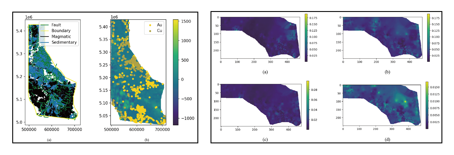
Take the Idaho dataset as an example, we can extract the features and mask data from this dataset by reading all the corresponding file (the mask indicate the intereted areas),

# Load feature geochemical data
feature_dict = {}
for feature in feature_list:
    rst = rasterio.open(data_dir + f'/{feature_prefix}{feature}{feature_suffix}')
    feature_dict[feature] = rst.read(1)

# Load mask raw data and preprocess
mask_ds = rasterio.open(data_dir + f'/{mask}').read(1)
mask = make_mask(data_dir, mask_data)

# More features added and filtered
if feature_filter:
    dirs = os.listdir(data_dir + '/TIFs')
    for feature in dirs:
        if 'tif' in feature:
            if 'toline.tif' in feature:
                continue
            rst = rasterio.open(data_dir + '/TIFs/' + feature).read(1)
            if rst.shape != mask.shape:
                continue
            feature_list.append(feature)
            feature_dict[feature] = np.array(rst)

Then, we can process the labels by dealing the deposite files in this dataset,

# Load label raw data
label_x_list = []
label_y_list = []
for path in label_path_list:
    deposite = geopandas.read_file(data_dir + f'/{path}')

    # Whether to filter label raw data
    if label_filter:
        deposite = deposite.dropna(subset='comm_main')
        au_dep = deposite[[target_name in row for row in deposite['comm_main']]]
    else:
        au_dep = deposite

    # Extract the coordinate
    label_x = au_dep.geometry.x.to_numpy()
    label_y = au_dep.geometry.y.to_numpy()

Afterwards, four stages are included in the next data pre-processing pipeline: auto-interpolation, feature filtering, data enhancement and data split. These are done in an automatical way to reduce users’ overhead,

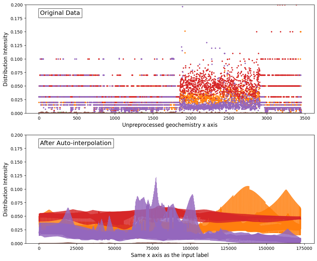
Auto-Interpolation

The selection of different interpolation strategies in method.py.

• scipy.interpolate.interp2d with interpolation kinds of [‘linear’, ‘cubic’, ‘quintic’].

• pykrige.OrdinaryKriging with interpolation kinds of [“linear”, “gaussian”, “exponential”, “hole-effect”].

Note

Only some datasets need interpolation process and Idaho does not need that. AutoMPM will judge automaticall weather it is required for interpolation.

# pre-process the x-y grid that we have to do interpolation
x_geo, y_geo = geochemistry.geometry.x.values, geochemistry.geometry.y.values
x_max, y_max = mask_ds.index(mask_ds.bounds.right, mask_ds.bounds.bottom)
z = geochemistry[feature].values

# interpolation optimization
interpOPT = interp_opt()
result = interpOPT.optimize(x_geo, y_geo, z, x_max, y_max)

Automated selection entails favoring the method with the lower Mean Squared Error (MSE) loss value or higher performance metric sore (F1 score etc.), thus designating it as the introductory technique of choice. The default choice of criterion is MSE loss.

Feature Filtering

Then, an automated two-tier screening workflow is used in autoMPM. In the first tier, the system filters the features based on their Pearson coefficient with the training labels. In the second tier, the system employs Shapley values, which provide a systematic measure of the contribution of each individual feature to the overall model performance.

• Feature_Filter.get_shapely a highly integrated function that output the Shapley vlaue with assistance of a random forest classifier.

• Feature_Filter.select_top_features automatically select the top-k features. k is set default to 20.

feature_filter_model = Feature_Filter(input_feature_arr=feature_arr)
feature_arr = feature_filter_model.select_top_features(top_k=20)

Data Enhancement

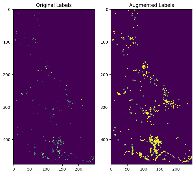
Data augmentation was employed to expand each ore spot from a single point to a mxm area, which allows for a more comprehensive representation of the ore distribution, capturing the spatial context and potential variations within the surrounding area.

• augment_2D assign the m*m blocks around the sites to be labeled. m is set default to 3.

# save the original label for test set
ground_label_arr = label2d[mask]

# data enhancement
label_arr2d = augment_2D(label_arr2d)
label_arr = label_arr2d[mask]

Data Split

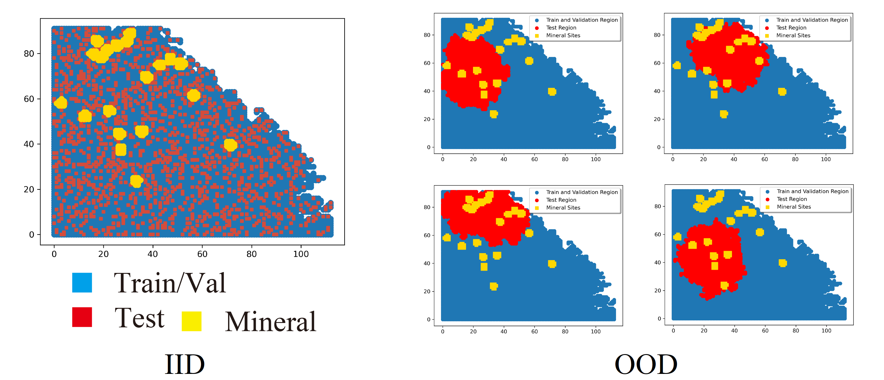
• Two data split ways that suitable for different situations:

  • (IID) Split by random-split strategy.

  • (OOD) Split by K-Means clustering algorithm with a scheme to choose a certain start point of generating subarea to cover all splitting scenarios with fewer trials.

• random_split for IID case. Split the dataset into train set and test set, and apply K-fold Cross-validation.

• dataset_split for OoD case. Split the dataset using K-means clustering, as in test_extend that generate the mask of test dataset.

# IID
if self.mode == 'random':
    dataset_list = self.random_split(modify=self.modify)
# OoD
else:
    test_mask, dataset_list = self.dataset_split(test_mask, modify=True)

Note

The data split operation is typically executed in the predicting stage, but for the purpose of this code example, it is included as a pre-processing module.

After all the pre-processing stages, the raw data will be packed in a .pkl file:

# Pack and save dataset.
dataset = (feature_arr, np.array([ground_label_arr, label_arr]), mask, deposite_mask)
with open(output_path, 'wb') as f:
    pickle.dump(dataset, f)

Algorithm and Hyperparameter Selection

Bayesian Optimization Auto-ML system

After pre-processing, the data package is input into the automatic system. It’s driven by Bayesian Optimization which will choose and optimize and best algorithm and its corresponding hyperparameters. Here we adopt a parallel and multi-fidelity accelerated design in our auto system.

The output of AutoMPM comes from its algorithmic predictions. The algorithm class used for mineral prediction is shown below: (here taken the rfc algorithm as an example)

class rfcAlgo(RandomForestClassifier):
    DEFAULT_CONTINUOUS_BOOK = {}
    DEFAULT_DISCRETE_BOOK = {'n_estimators': [10, 150], 'max_depth': [10, 50]}
    DEFAULT_ENUM_BOOK = {'criterion': ['gini', 'entropy']}
    DEFAULT_STATIC_BOOK = {}

    def __init__(self, params):
        super().__init__(**params)
        self.params = params

    def predictor(self, X):

        pred = self.predict(X)
        y = self.predict_proba(X)
        if isinstance(y, list):
            y = y[0]
        return pred, y[:,1]

• __init__(self, params): Initialize the algorithm with parameters, unpacking them to the super class.

• predictor(self, X): Unveil 2-class results and probability predictions for sample classifications.

Hyperparameter Constraints

AutoMPM ensures sound hyperparameter tuning by adhering to these constraints:

• Continuous Param: Lower and upper bounds as a floating-point list of length 2.

• Discrete Param: Lower and upper bounds as an integer list of length 2.

• Categorical Param: Enumeration of feasible options within a list.

• Static Param: A static value serving as a constant.

Example Use

# Automatically decide an algorithm
algo_list = [rfcAlgo, extAlgo, svmAlgo, NNAlgo, gBoostAlgo]
method = Method_select(algo_list)
algo = method.select(data_path=path, task=Model, mode=mode)
print(f"\n{name}, Use {algo.__name__}")

# Bayesian optimization process
bo = Bayesian_optimization(
    data_path=path,
    algorithm=algo,
    mode=mode,
    metrics=['f1', 'auc'],
    default_params=True
)

x_best = bo.optimize(300, early_stop=50)

Summary

Prepare to embark on your AutoMPM journey by following these steps:

1. Preprocessing: Use the functions in data_preprocess.py to preprocess your raw data effectively.

2. Hyperparameter Mastery: Understand the constraints governing hyperparameter tuning.

3. Run the Code: Before executing the system, ensure you update the file path in test.py.

4. Check the Output: The output will be recorded in a .md file in run folder.

With the AutoMPM toolkit, you can accelerate the mineral prospectivity mapping endeavors with automation, precision, and enhanced insights. Let AutoMPM be your assistant for efficient exploration.

Bayesian Optimization in AutoMPM

Optimization Logic

The logic workflow of hyperparameter optimization in optimization.py.

• Automatically choose the best hyperparameters for the machine learning algorithm.

• Multi-processing on multiple threads to accelerate the predicting process. It simultaneously evaluates multiple parameters in parallel, aggregates results and proceeds to the next iteration.

• Employing a multi-fidelity strategy, an initial low-fidelity estimation is conducted using a weighted cross-entropy metric. If performance surpasses a set threshold, a high-fidelity estimation is executed for refinement.

• data_path: Specifies the path to the dataset used for optimization.

• algorithm: Specifies the machine learning algorithm or model used for optimization.

• mode: Indicates the optimization mode or strategy.

• metrics: A list of evaluation metrics, including ‘f1’ (F1 score), ‘auc’ (Area Under the ROC Curve), ‘pre’ (precision score), used during optimization.

• default_params`: Implies that default hyperparameters are initially used for optimization.

# Initialization
X, y, names = self.initialize(x_num)
if early_stop == 0:
    early_stop = steps
early_stop_cnt = 0

# Find the best in initialized samples
best = np.argmax(y)
y_best = y[best]
name_best = names[best]

# Optimization iterations
for step_i in range(steps):
    x_sample, name = self.opt_acquisition(X)
    y_ground = self.evaluate_parallel(name, self.worker)
    worker_best = y_ground.argmax()
    name = name[worker_best]
    x_sample = x_sample[worker_best]
    y_ground = y_ground[worker_best]

    # Check whether this is the best score till now
    flag = False
    if y_ground > y_best:
        y_best = y_ground
        name_best = name
        early_stop_cnt = 0
        flag = True

    # Early stop
    if not flag:
        early_stop_cnt += 1
        if early_stop_cnt == early_stop:
            break
    else:
        early_stop_cnt = 0

    # Update the surrogate function
    self.gaussian.fit(X, y)

Process of Hyperparameters

The format of hyperparameters that input, store, and use in optimization.py.

• Change the input of hyperparameter info into a fully dict-like format, as:

• param_name: {

  • type: Enum(continuous,discrete,enum,static)

  • low: float or int

  • high: float or int

  • member: IntEnum(#member)

  • value: float or int

  • }

• An encapsulated function for checking the format of hyperparameter info - Whether in the params of the algorithm - Continuous and discrete: low and high - Enum: member - Static: value

• An encapsulated function for translating between hyperparameter info and value type - Continuous to uniform - Discrete and enum to randint

Method Selection

The selection of different machine learning methods in method.py.

• Evaluate each method with steps in low-fidelity Bayesian optimization, and choose the one with the best performance.

class Method_select:
    def __init__(self, algorithms=[rfcAlgo, NNAlgo]):
        self.algos = algorithms
        self.best_algo = None
        self.opt_score = -100

    def evaluate_algo(self, algo, data_path, task, mode):
        # low-fidelity estimation for method selection

        bo = Bayesian_optimization(data_path, task, algo, mode=mode, default_params=True, fidelity=1, worker=3, modify=True)
        best, X, y = bo.optimize(steps=5, out_log=False, return_trace=True)
        score = np.mean(y)
        print(f'{algo.__name__}, score: {score:.4f}')
        return score

    def select(self, data_path, task, mode):

        with concurrent.futures.ThreadPoolExecutor(max_workers=16) as executor:
            future_to_algo = {executor.submit(self.evaluate_algo, algo, data_path, task, mode): algo for algo in self.algos}

            for future in concurrent.futures.as_completed(future_to_algo):
                algo = future_to_algo[future]
                try:
                    score = future.result()
                    if score > self.opt_score:
                        self.best_algo = algo
                        self.opt_score = score

                except Exception as exc:
                    print(f'Error while evaluating {algo.__name__} Model: {exc}')

        return self.best_algo

Appendix

Algorithms

The algorithms to build a model for mine prediction.

• More encapsulated algorithms and corresponding default hyperparameters in algo.py:

  • Logistic Regression (LGR)

  • Neural Network (NN)

  • Support Vector Machine (SVM)

  • Random Forest (RF)

  • Extra Trees (ET)

  • Gradient Boosting (GB)

  • Random Forest Boosting (RFB)

  • SVM Boosting (SVMBT)

  • LGR Boosting (LGRBT)

  • SVM Bagging (SVMBG)

  • LGR Bagging (LGRBG)

  • NN Bagging (NNBG)

  • Extreme Gradient Boosting (XGB)

  • Light Gradient Boosting (LGB)

Code Files

Code structure of AutoMPM:

• optimization.py: Bayesian optimization

• constraints.py: Encapsulation of hyperparameter settings

• model.py: The model of auto machine learning algorithm

• algo.py: Encapsulation of algorithms

• method.py: Automatically select the algorithm

• utils.py: Some tool functions

• data_preprocess.py: Data pre-process

• metric.py: Shapley value tool

• interpolation.py: The optimization for interpolation

• test.py: The template code to run